Load Cell Probing Algorithm Testing

[garethky]

@alexb

@garethky If you take the average between the elbow and elbow-1, wouldn’t that be sufficient?

You know what, that’s a gem, that’s a really good guess .

The collision point is randomly distributed between [elbow, elbow-1] because its based on the timing of the collision and the sensor reading, which we cant control.

bogo does so well because the distance between any 2 random points on a line is 1/3. Guessing the middle point gets you down to an average error of only +/- 1/4.

Guessing like this is using only the elbow point. It just feels like there should be some way to use the rest of the points to make a guess. So that’s why I’m looking bspline, its the only one so far that can outperform a guess. I haven’t tried it in the printer yet but I have high hopes.

I also haven’t gotten there yet but stacking is worth trying. If linear regression comes up with an answer outside the [elbow, elbow-1] range, try bspline and if that also fails just guess the middle. That would curtail the worst of the outliers but preserve the good performance in linear and “near linear” conditions.

I’m busy adding the elbow finder testing as well…

[garethky]

@leadinglights do you have graphs of this stuff? Like what is the shape of a collision for your setup?

If this was CAD I would draw some lines and connect them with tangency constraints. Then I could parameterize the radius, length, angle and so on. I’m not sure how to do that easily with just python.

Capturing data and re-using it wont allow me to change parameters easily. E.g. the data changes with the timing of the collision and the sensor sample time. I need so simulate a range on those conditions to properly test the algorithm.

I have considered doing fits of logged data with something like bspline to extract reusable test collisions but haven’t tried to implement it yet.

[leadinglights]

First picture is a trace from a 27mm piezoelectric disc with a simulated contact at only 1mm/sec. This trace is my favorite as it was the very first trace I got and I expected only some tens of milivolts but got 8.0V. More details on Piezoelectric disks for Z contact detect and bed levelling. The decay after the peak is somewhat faster than I would have expected, but I now think that this is a result of elasticity in parts of the jig - this would also account for the acceleration in the mid part of the upstroke.

The second picture shows three repeats of a 2mm per second nozzle contact on a glass plate with a Kapton film. Each trace is the sum of the output of three piezo discs in an underbed arrangement and each is the pre-trigger data in the 32ms before contact. The trigger was set artificially high to see what was happening. This picture is from the same forum thread, but on the last page.

There is a little more on Report on under bed sensor problems but this thread is mostly about finding that any kind of underbed sensor has problems.

Mike

[garethky]

I like that, I REALLY want a oscilloscope!

It looks really linear, but if you put a straight edge next to it, you see its actually increasing:

My guess is backlash? The toolhead goes from being loaded by gravity to loaded by the build plate. All the bearings switch which contact faces are loaded and they all have some lash.

Outside that, the axes are non-linear at small scales as well. Good ball screw manufacturers have a spec for this, e.g. https://tech.thk.com/en/products/pdf/en_a15_011.pdf

They have this diagram that shows the fluctuation of the linear ball screw:

But in a 3D printers we use usually use lead screws, pulleys, bushings and belts. There is little spec data available for those but I’ve seen as high as 0.2mm over 300mm for the repetitive travel distance error on a lead screw (at least in reputable places that have specs). The fluctuation is nearly equal to the total in the THK data sheet for short lengths. Its not much on the 0.05mm length scale but it should be detectable

@leadinglights

btw, I use Savitsky-Golay in the “monkey see monkey do” mode - I don’t understand it, but it works.

Filtering is something I really want to test out in this simulator. I tried a couple of things on the printer but it was inconclusive. My sample sizes are just too small.

[leadinglights]

You may well be right about the backlash, but this does leave me with a bit of a quandary: If it is backlash then the decay after the peak is faster than it should be for the capacitance of the piezo and the input resistance of the scope. If however, the acceleration is due to the moving mass of the jig bouncing, then the peak is an artifact and the real value is closer to 6V and the decay is about right.

On the filter, I have attached a plot of raw data, filtered data used for finding the trigger, and SG 9-point slope data. I think the regular fluctuation on this is from the stepper motor driver.

The trigger is generated from the mean of 8 points while the slope is used as part of the good/bad criteria.

Mike

[garethky]

If you can see stepper motor pulses you must have the sample rate turned up WAY higher than we will be able to handle. Seems right, its too fast for 60Hz noise.

For filtering, because I’m only trying to do this after the collision occurs, I don’t need to filter on the MCU in real time. For real time applications you have to use only previous data points to filter. But for captured data you can use points in both directions. Using only previous data points introduces a lag (“phase delay”) between the filtered value and the real value. But if we use a forward/backward digital filter it will have no lag, see example here: scipy.signal.sosfiltfilt — SciPy v1.11.1 Manual

This is the advantage of the python post analysis approach, we can use the best technique for the job, even if its slower or impractical in a real time system.

Slope through n points is an interesting metric. That’s basically the derivative, the rate of change. I’ve read some examples of that technique being used to find the elbow in a plot. In your example the exact elbow is really ambiguous but that technique does a good job of putting upper and lower bounds on it.

The width of that could be useful in classifying good vs bad taps. Based on everything I have tried, we want to reject “soft” elbows. A soft elbow is what something squishy under the nozzle looks like. 30x^2 in the test set is very clearly a soft elbow.

[garethky]

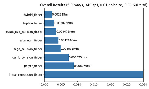
@Alexb I added your “mid” finder as dumb_mid_collision_finder and the idea of cascading multiple algorithms as hybid_finder.

Here with no noise, the strategies that assume there is some information in the data perform best. This gives you a good idea of the natural rank of the guess based finders.

But with added noise the hybrid approach is able to win:

dumb_mid_collision_finder even beats the estimator finder!

This is encouraging. I’m going to try adding smoothing to the bspline_finder to see if I can bring its performance on noisy data close to the no-noise case. We should be able to pick the right smoothing settings by looking stats or an FFT on the data before the collision.

[garethky]

Elbow Finding

So far we have not discussed this topic and its very important. The *_finder implementations above rely on the elbow finder algorithm to identify where in the sequence the collision data set begins.

The current code uses an algorithm that I copied from the Prusa source code. It works like this:

• break the data into 2 data sets, left and right
• calculate least squares for left and right
• sum the residuals (the squares of the distances to the line of the points)
• Move the left/right split point backwards through the array until the sum of the residuals hits a minimum.
  This has the distinction of shipping in a commercial product so lets see how we get on:

linear_regression_elbow_finder, No Noise vs Noise 0.01

Reading the charts: The units are how many array positions the finder’s guess is away from the true value, on average. A perfect score would be 0. If the bar is to the right of the zero line the guess is to the right of the true elbow index, left means the opposite. A value over 1.0 is likely going to cause a major degradation in accuracy.

So this version works well on the linear function 50x but for anything else its giving unreliable results. I thought about this a bit and I read through @D4SK’s implementation. That code has the idea of dividing the residuals on the right/collision side by the number of points in the right line. (There are a lot of other ideas there, but a lot of them use magic numbers which I cant really generalize to other peoples printers). This algorithm is basically a kind of gradient descent and the sum of the residuals is a cost function. Making the cost of the residuals on the right less expensive for curvy data should encourage greedier behavior:

So linear_regression_ratio_elbow_finder has a cost function of left_residuals + (right_residuals / (len(right_line)):

So this is a pretty big improvement in the no noise case. So maybe some further ideas about optimizing that cost function would get us closer to a perfect score.

The last thing I tried is the algorithm describes in this paper from Satopaa et al. called “Kneedle”. Kneedle is based on the idea that the points of maximum curvature in a data set, the knees/elbows, are the set of points in a curve that are local maxima if the curve is rotated clockwise about origin through the line from its beginning to its end. Its a simple idea and its much faster to calculate than recursive calls to least squares:

I’m shocked that’s so good! I bet that performs better than my eyeball. It has a usable score on everything but 30x^2. I would argue that 30x^2 should be rejected because it looks exactly like the nozzle hitting hot plastic blob.

It tends to guess negative. It seems logical to add 1 to its guess so we don’t include points from the horizontal part of the data in the set used to find the exact collision point. So this is the new winner for elbow finding.

The next thing to explore here is what characteristic of the Kneedle height values would indicate that the knee/elbow is too soft to accept. Maybe the derivative of this data would reveal something usable.

[leadinglights]

The sample rate is 4000 samples per second. Fortunately, the circuitry and implementation don’t suffer from mains interference (50Hz in the U.K.) but mechanically introduced mains frequency hum is catastrophic.

The slope is found by looking ahead by four samples and back by four samples so that the slope on the graph matches up pretty well with the raw data. The mean of 8 samples on the other hand is generated from the past 8 data points so is later which can be seen in the green trace being displaced to the right.

The knee finding is very unsophisticated as it is found simply by looking at a mean of 8 ADC values from a set time before the trigger value was passed - in the given graph this may be about 20ms back. The closer it is to the baseline the sharper the knee. Where the sample is taken should be taken will vary with the slope of the line, but a fixed position gives really quite acceptable discrimination of soft knees.

As to how acceptable: Hot soft plastic on the nozzle is always detected and cold softer plastics such as ABS can be detected at a thickness greater than about 0.5mm. Cold PLA on the nozzle is not easily detected even at thicknesses > 1mm. At the upper limit, a greasy fingerprint on a glass bed can be detected by a touch version of the piezo probe. The greasy fingerprint prize winner is the second touch probe shown on Thoughts on a piezo touch sensor Please disregard the last two probes pictured as they are disappointments to their parent.

I looked at the Satopaa paper but I think it fried my brain.

Mike

[garethky]

@leadinglights

I looked at the Satopaa paper but I think it fried my brain.

Its long and they go into their particular application for it which we don’t care about. But early on there is a nice diagram of what they are doing that I was able to grock.

I tried the +1 idea and that works well. So maybe there are conditions where I should add 1 and some where I should not? My first guess is this:

if (delta_y[elbow_index - 1] < delta_y[elbow_index + 1]):
    elbow_index += 1

The idea is you’d expect the Y value to drop faster in the collision set, so if that’s not the case, add 1.

That version, in the no-noise condition, performs significantly better than just adding 1. It actually gets a perfect score on 3 of the functions:

Looking at plots of the Kneedle distances for incorrect answers, some I can see with my eyeball are wrong:

and some I cannot tell at all:

Performance in no-noise conditions is important because its a good predictor of the ceiling of performance when real data is smoothed.

So my next idea is computing the perpendicular distance of the selected elbow point from the lines either side of the elbow. If its closest to the left line, the approach line, then add one. In the no noise case that works perfectly:

It turns out the line to the left can go all the way back to the beginning of the plot, but the line to the right has to be shorter. I used 10 points but we often have fewer than that which seems to be fine. With noise it doesn’t perform any better than my first guess. I likely need noise filtering to improve this.

If you have another idea for this “when to +1” condition I’m all ears.

[garethky]

Started algorithm testing on the actual printer. Doing batches of 50 probes at 1, 2, 5, and 10mm/s. Wanted to re-create the Euclid probe accuracy plots and got this…

I have no explanation for that sawtooth pattern! It was in the data before I started changing code and after. Its less pronounced at lower speeds, but still there.

Maybe:

• Some sort of issue with the tool changer mechanism? Like it gets pushed and then slips back?
• Timing issue?
• MCU clock drift?

[koconnor]

I’m not sure what is causing the saw tooth pattern. (I’m also not fully understanding the test and design strategy you are perusing here.)

However, if you are looking to calculate very accurate toolhead positions (eg, microns), then you’ll need to calculate the precise stepper positions at the time of the event. The requested toolhead position (eg, trapq_extract_old) is unlikely to provide sufficient precision. In particular, the step compression code can move each step time to within a window of 25us, and depending on the Z stepper step size, that alone can result in measurable deviations of the calculated position.

You can look at how klippy/extras/homing.py handles this (in particular how it tracks the halt time separately from the trigger time and how it calculates the stepper positions from the trigger_time and then calculates the cartesian trigger position from those stepper positions).

Cheers,
-Kevin

[koconnor]

For what it is worth, I’m not sure I agree with the testing methodology described here (nor do I fully understand it). I would, however, caution to be careful with mixing “accuracy” goals with “repeatability” goals.

I’d argue that the primary goal of homing and probing is “repeatability”. Accuracy isn’t actually a particularly important goal at all.

Said another way, if I home a printer and move to a position of x=50, y=50, z=50, and repeat that process a thousand times, then I really really want the printer to be in the exact same position all one thousand times. That is, the distance between toolhead and bed should be the same, the distance between toolhead and frame should be the same, the pulleys (or rods) on every stepper should be in the same angle, every stepper motor should be in the same phase, etc. It is not actually important that the toolhead be exactly 50mm away from the bed or 50mm away from the frame.

This “repeatability” is important, because if I can get the printer repeatable, then I can easily fix for any inaccuracy by measuring that inaccuracy and add an appropriate static offset. So, if the above procedure repeatably moves the toolhead to 52.003mm from the bed, then I can add a 2.003mm static adjustment and then I’ll then have repeatable accuracy.

In contrast, accuracy without repeatability doesn’t provide much value. For example, if in the above example, I get a very “accurate” homing process that leaves the toolhead sometimes at 50.020mm, sometimes at 49.990mm, and sometimes in between those points, then I have much worse results in general. That is, although the accuracy is dramatically better in this example, the actual utility is dramatically worse.

So, for what it is worth, any kind of load cell probing inaccuracy is only relevant if it is not a repeatable inaccuracy. I would keep that in mind when designing any algorithms.

Cheers,
-Kevin

[garethky]

@koconnor

However, if you are looking to calculate very accurate toolhead positions (eg, microns), then you’ll need to calculate the precise stepper positions at the time of the event. The requested toolhead position (eg, trapq_extract_old) is unlikely to provide sufficient precision. In particular, the step compression code can move each step time to within a window of 25us, and depending on the Z stepper step size, that alone can result in measurable deviations of the calculated position.

I have implemented an endstop that overrides home_wait() and returns an exact time that the collision started. This should be leveraging all the goodness in HomingMove.homing_move() that works out exact stepper positions.

Since what I’m returning is a print time, any time skew would result in a z position skew. At least it looks like that kind of problem.

I’m using PROBE_ACCURACY to run the tests in batches of 50. I would have thought that each probing attempt would have compressed to the same instructions, so that shouldn’t be a source of variance here?

The Z axis on the test machine is a bit of a mutant, ball screw + belt drive:

rotation_distance: 4  # The ball screw moves the Z axis 4mm for 1 rotation
gear_ratio: 36:17     # reduction pulleys used to drive the ball screw
microsteps: 16
full_steps_per_rotation: 200

I believe that’s ~105.8 full steps per mm and ~1694.1 microsteps per mm. So 0.009mm for a full step or 0.0006mm per microstep. 25us is ~2 microsteps @ 5mm/s. At 400sps and 5mm/s each measurement is 2500us appart, or 0.0125mm/20 microsteps.

I agree about repeatability 100%. That is the goal. I saw cases that clearly represented non-real results that would lead to a lack of repeatability. The difficulty is that they are based on the timing of the probe and the sensor samples. So using a test tool like this allows me to see those cases in a repeatable way and find solutions that performs in a predictable way in all conditions.

Said another way, if you get an improved average, SD or range on PROBE_ACCURACY it might be because your timing was just lucky. Reproducing the unlucky cases at will on the printer isn’t practical. A synthetic benchmark can always include those cases.

I don’t really want to report results too early because of this sawtooth business.

[koconnor]

@garethky

This should be leveraging all the goodness in HomingMove.homing_move() that works out exact stepper positions.

Okay - if you’re using the stepper position already then that is great. I know in another thread you asked about trapq_extract_old, so I wanted to make sure you were aware of the limitations of that mechanism.

@garethky

Since what I’m returning is a print time, any time skew would result in a z position skew

If the sensor and stepper are on the same MCU then I don’t think clock synchronization would alter the results - as the conversion from mcu_clock to print_time back to mcu_clock should not be lossy. (That is, any clock skew should fallout.)

If the sensor is on a different MCU then clock synchronization can introduce a deviation. This is a known limitation of “multi-mcu homing”. Typically Klipper does a good job of synchronizing clocks, but you can graph the results of the logs ( Advanced Trouble-Shooting / Graphing Klipper ) if you want to investigate that.

-Kevin

[garethky]

@koconnor

I know in another thread you asked about trapq_extract_old, so I wanted to make sure you were aware of the limitations of that mechanism.

Ahh, yeah I was trying identify samples between the endstop trigger and the actual stopping of the axis. Those samples potentially useful for regression. I haven’t included this yet as its a lot of code and the data may be of dubious value as it tends to be non-linear anyway.

@koconnor

If the sensor and stepper are on the same MCU then I don’t think clock synchronization would alter the results

It is a Multi-MCU setup, but the sensor and the steppers are on the same MCU. Still that’s a variable I could eliminate.

Things on the TODO list:

• look at graphstats.py output
• Remove MCU #2 from the printer’s config
• Try the same test with the z endstop as a probe and see if it reproduces (excludes my code + toolchanger mechanism)
• Try mounting a switch probe to a tool holder and see if that reproduces (excludes just my code)
• Try aggressively oversampling the sensor (e.g. 40Khz) and reporting exact 32 bit clock time for reads.

Cheers, thanks for the help

[garethky]

Switch based probe on the carriage shows no sign of the sawtooth.

Repeatability of this z-axis (50 probes, 5mm/s):
// probe accuracy results: ... range 0.001181, standard deviation 0.000416
I picked this setup for testing because I expected it would be more repeatable than most printers out there. The standard deviation is just below 1 microstep.

But if I had to place a bet, the root cause has to be in my code. That’s just the tyranny of writing software. So, skipping to the last debugging step on the list… Returning 32bit clocks from the MCU instead of the clock dead reckoning:

Sawtooth is gone . Another clue is that the clock roll over on this MCU is ~23 seconds and that pretty much lines up with the sawtooth times in the graphs. The clock dead reckoning must be diverging somehow.

No specifics yet because the outliers in that chart are exactly what I’m trying to fix. But this is a real improvement!

[D4SK]

Great work! Cannot read through everything right now. But i wanna make one point about the dynamics.

Basically the printbed acts like a mass between two springs, (printhead mount, and printbed mount) one of the two springs includes the strain guage. before the collision the printbed has 0 velocity, or full probing velocity(depending on printer). If we assume both springs have the same stiffness the printbed will accelerate or decelerate to have 0.5*probing_velocity during the contact phase.

Let’s assume the printhead is a lot lighter than the buildplate.
This acceleration or deceleration causes a nonlinear behaviour. When mesuring force above the printhead it will be a bump, with momentarily higher deflection(force) at the load cell.
If we measure the force below the bed, the opposite will occur, and it will gradually acellerate before showing a deflection.

Here are my measurements with 3 load cells (5k, hx711) below the printbed.

[garethky]

I am trying to use all the the algorithms to analyze a group of 50 probes logged on the test printer. So far none of the algorithms has standout performance. The best that any of the elbow finders can do is about 80% “correct”.

I say “correct” in quotes because I don’t have an Oracle to tell me the exact contact time. There for I cant say for sure if any particular result is true. I have spent about 2 days trying to build a way to see if a group of elbow results look like they could be correct.

The tool I came up with is to visualize the z coordinates of the selected elbow and the point before the elbow. So each vertical blue bar is the z distance between the 2 samples. I expect that the true z coordinate should be within that band of all probes if the elbows are all well selected.

If I sort the probes buy Z coordinate this makes more sense:

That red line is the likely true z coordinate.

If I plot the delta in force between elbow - 1 and elbow in the same order as the sorted probes, I expect that I will see some sort of coherent function. Basically a longer time before reporting the sample should result in more force and higher reading at the sensor. And when I do this I see:

Its “linear-ish”, noisy but its certainly not random. It’s at least linear enough that making a guess based on the ratio of the force delta outperforms making a guess at the midpoint:

Guess Midpoint       -- range: 0.0124, standard deviation: 0.0039, average: 1.5573
Elbow Force Ratio    -- range: 0.0025, standard deviation: 0.0007, average: 1.5717

But getting that quality of results required hand correcting some of the results for elbow guesses. So I could just be fooling myself.

For automated elbow detection, the Kneedle algorithm is still better but its only about 80% reliable:

Doing the same trick to plot the force offsets of the above shows a clear discontinuity which makes me strongly suspect these results are not consistent with a true physical reality:

[garethky]

Thanks, I wanted people to see those plots. I think that might not be atypical of some printers.

There are maybe 15 points in that elbow. Its no sharp. I don’t know if we can offer any kind of repeatability with that kind of curve. Where the green line ends up is very dependent on which points get included in the linear regression. And if you don’t use enough points the result ends up being late, which translates to too low.

Whereas on my machine (at least at 5mm/s / 400SPS) I get really sharp elbows. Maybe 1 point in the elbow, maybe zero.

After my investigation this weekend I am ready to give up on using the post collision points for anything. Any math I do with them works out to have a higher range & SD than if I only use the first point in the collision.

I need to re-run my investigations at 2mm/s @ 400 SPS and 5mm/s @ 1200SPS. I think those may be more sane samples/mm values (0.005mm and 0.004mm). At those speeds I should start seeing soft elbows like yours.

We can also look at the retraction. That’s actually what Prusa are doing. That method doesn’t work well with the order of operations in klipper. But in your plots you can see the retraction line overshoots the x axis and provides a less ambiguous linear regression.